⚡ Chile Energy Grid Forecasting

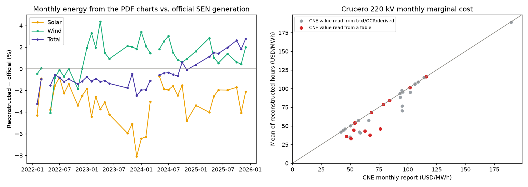
Hourly forecasting of Chile's National Electric System (SEN) on four years of real hourly data (2022-2025): marginal cost at 6 real 220 kV buses from Antofagasta to Puerto Montt, and system-wide solar generation, wind generation and demand. The hourly series are not downloaded from an API (the grid coordinator's requires an institutional account): they are read out of the vector charts in the coordinator's public daily PDF reports, calibrated day by day against the numbers each report prints, and validated against two independent official monthly series. On top of that: LightGBM tuned with Optuna and validated walk-forward against naive baselines, real weather features (ERA5), Rolling-Origin CV against XGBoost, a PyTorch MLP, conformal prediction intervals, a recursive multi-step forecaster and a Streamlit dashboard.

Code and method Full README

This page shows the project's results. The methodology, the design decisions and the limitations are documented in the repository's README.

2. Data: four years of real hourly data, read out of PDF charts

Reconstruction vs. official monthly series — - **Monthly energy vs. the official SEN generation (datos.gob.cl):** total within 3% (usually 1-2%), wind within 5%. Solar from the charts is consistently 2-8% *below* the official series: the two sources do not count exactly the same plants. - **Crucero's monthly marginal cost vs. the CNE monthly reports:** from June 2022 to June 2024 the mean of the reconstructed hours matches the CNE figure to within about 0.5 USD/MWh. **From July 2024 the two publications diverge**: the daily report is 9-30 USD/MWh lower than the CNE figure every month.

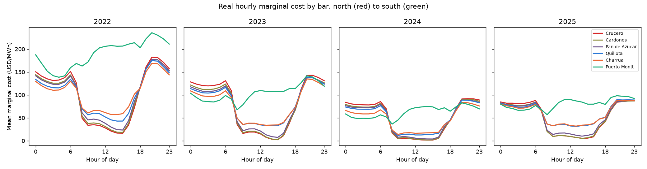
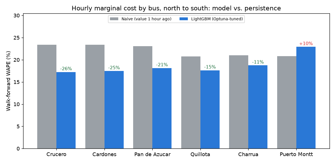
Real hourly marginal cost by bus — **The price splits by geography at noon.** Between 10:00 and 16:00, Crucero, Cardones and Pan de Azúcar sit below 1 USD/MWh in 70-74% of hours (solar surplus in the north), Quillota and Charrúa in 53-56%, and Puerto Montt in only 29%. The system's residual demand correlates 0.64-0.73 with the price at five buses and 0.19 at Puerto Montt (`notebooks/01_eda_seasonality_analysis.ipynb`): one system-wide driver does not price a bus that transmission isolates.

5.1 Walk-forward validation: LightGBM (Optuna-tuned) vs. baselines

Price WAPE by bus: model vs. persistence — **The model's edge shrinks from north to south and turns negative at Puerto Montt.** In the north, the noon price collapse is predictable from the system's solar and the hour of day, which persistence cannot see coming. Puerto Montt's price is barely related to the system's residual demand (correlation 0.19, §2), so the features that carry the other five buses do not help it, and one model shared across buses applies the northern pattern where it does not hold. A per-bus model or bus-specific drivers (regional hydro, transmission limits) would be the next step there.

5.4 A third modeling family: PyTorch MLP vs. LightGBM/XGBoost, and ReLU vs. GELU vs. Swish

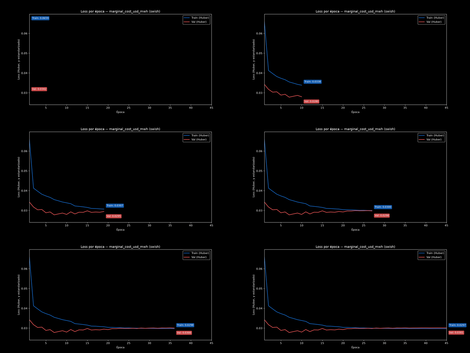
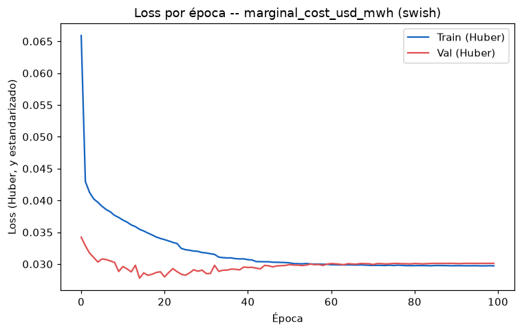
A dense MLP with a custom Huber loss, trained on the same folds and features as the tree models. On the old simulated panel it was the best model on price; on real prices every activation lands at 21.7-22.0% WAPE, above default LightGBM (19.9%) and level with persistence (21.9%). All 15 runs reach their best validation loss between epochs 8 and 21: the network starts overfitting real prices almost immediately.